How to Effectively Find the Interquartile Range in 2025: A Practical Guide to Data Analysis
The **interquartile range** (IQR) is a critical measure in statistics that helps in understanding the variability and spread of a data set. This guide will delve into the **definition of interquartile range**, methods of **calculating interquartile range**, and its importance in **data analysis**. We will explore practical steps to find the **interquartile range**, supplemented with real-world examples and graphical representations to enhance understanding.
Understanding Interquartile Range: Definition and Importance
The **interquartile range** is defined as the difference between the upper quartile (Q3) and the lower quartile (Q1) in a data set. It measures the middle 50% of the data, effectively capturing the range of values that lie between the first and third quartiles. This measure is significant as it offers insight into areas where data clustering occurs, and it actively filters the influence of outliers, presenting a clearer representation of the data’s dispersion. Understanding the **importance of interquartile range** is crucial for those engaging in extensive **statistical analysis**.
Importance of Interquartile Range in Data Analysis
The **interquartile range** plays a pivotal role in various contexts. For instance, in the realm of descriptive statistics, it provides an efficient means of assessing spread and variability without succumbing to the influence of outliers. Organizations often utilize the IQR to analyze employee performance data, sales trends, or any dataset requiring insights free of extreme values. Furthermore, it forms the basis of the concept of the five-number summary, which is fundamental in **data analysis** techniques.
Interquartile Range vs Range: Key Comparisons
An understanding of the differences between **interquartile range vs. range** is essential for accurate data assessment. The range provides a measure of the overall spread of the data (i.e., the difference between the largest and smallest values), while the interquartile range focuses on the middle 50%. The IQR gives a more robust overview of data variability as it disregards extreme observations. This distinction is particularly salient in datasets containing outliers that could skew the range significantly.
Application of Interquartile Range
In various fields including finance, healthcare, and education, the **application of interquartile range** can yield significant insights. For example, in a classroom, evaluating student test scores with the IQR helps educators identify whether performance disparities reflect a systemic issue or are mainly due to a few outlier scores. Thus, applying the IQR method provides a focused view beneficial for decision-making processes rooted in qualitative data analysis.
Steps to Find the Interquartile Range: A Simplified Guide
Finding the **interquartile range** involves several clear, reproducible steps that can be applied across various datasets. Here, we detail the **steps to find interquartile range**, enabling users to calculate it easily.
Step 1: Organize Your Data
<pBegin by sorting your data points in ascending order. This step is critical since quartiles are derived from a clearly delineated dataset. For example, consider the data set: 4, 7, 1, 3, 8. Once organized, our dataset reads: 1, 3, 4, 7, 8. In this case, sorting enabled accurate identification of the quartile positions.
Step 2: Calculate the Lower and Upper Quartiles
Subsequently, the next critical action involves finding the lower quartile (Q1) and upper quartile (Q3). To calculate **Q1**, select the median of the lower half of the dataset. For our example, the lower half is 1, 3, 4; thus, Q1 = 3. Conversely, for **Q3**, calculate the median of the upper half (i.e., 4, 7, 8); leading to Q3 = 7. Hence, we find our quartiles defined.
Step 3: Apply the Interquartile Range Formula
With Q1 and Q3 determined, the final step entails employing the **interquartile range formula**, articulated as: IQR = Q3 – Q1. In our example, IQR = 7 – 3 = 4. Therefore, the **finding interquartile range** of the dataset reveals a spread of 4, encapsulating the variability efficiently.
Graphical Representation of Interquartile Range
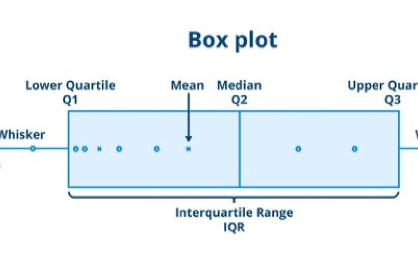
<pVisual representation of the **interquartile range** can further enhance understanding. **Box plots**, for example, effectively illustrate the distribution of data in relation to quartiles. In a box plot, the box spans from Q1 to Q3, visually distinguishing the interquartile range.
Understanding Box Plots
Box plots provide a significant visual interpretation of data spread via quartiles. The edges of the box correspond to Q1 and Q3, while a line within the box illustrates the median. Whiskers extend from the box to the smallest and largest data points that fall within 1.5 times the IQR from Q1 and Q3, respectively, effectively displaying potential outliers.
Real-World Example Using a Box Plot
Consider a scenario where an organization wants to evaluate its employee salaries. Upon creating a box plot and identifying Q1 as 30,000 and Q3 as 60,000, it becomes drastically evident that most employee salaries fall between these values (IQR = 30,000). Such visualization not only highlights salary distribution but also points out potential outliers, contributing greatly to informed decision-making processes.
FAQ
1. What does the interquartile range explain in a dataset?
The **interquartile range (IQR)** explains the middle 50% of a dataset, demonstrating how data points are clustered while filtering out the influence of outliers. It’s a crucial aspect of **descriptive statistics** that aids in understanding data spread and variability.
2. How do you calculate the interquartile range with an even number of data points?
For datasets with an even number of points, find the median of both halves. For instance, in the data set 2, 4, 6, 8, organize the data, identify Q1 (between 2 and 4) = 3 and Q3 (between 6 and 8)= 7. Then apply the formula: IQR = Q3 – Q1 = 7 – 3 = 4.
3. How does the interquartile range assist in detecting outliers?
The **interquartile range** assists in outlier detection by determining thresholds set at Q1 – 1.5 * IQR and Q3 + 1.5 * IQR. Any data points lying outside of this range are considered potential outliers, allowing researchers to maintain data integrity while performing analysis.
4. Can the interquartile range be used in all types of data sets?
Yes, the **interquartile range** can be effectively utilized in both continuous and categorical datasets where useful. This flexibility enables analysts across various fields to assess **data variability**, identify trends, and interpret results with considerable confidence.
5. How is the interquartile range relevant in advanced statistics?
The **interquartile range** becomes particularly relevant in advanced statistical applications by providing a robust measure of variability. When evaluating distributions, using the IQR helps analysts draw comparisons and substantive conclusions regarding the concentration and dispersion of data, which is vital in sophisticated research methodologies.
Key Takeaways
- Interquartile range (IQR) measures data variability while eliminating outliers’ influence.
- To calculate IQR, organize data, determine Q1 and Q3, and apply the formula IQR = Q3 – Q1.
- Graphical representations such as box plots offer visual insights into data distributions and implications of quartiles.
- The IQR is pivotal in statistical analysis, facilitating an understanding of trends and variability.
For further insights on data analysis and visual tools related to the interquartile range, consider visiting our articles here and here. Feel free to reach out for additional resources, and embrace the power of data mastery!